Introduction

To use shortcuts, you must include the following header:

#include "DGtal/helpers/Shortcuts.h"

And choose an appropriate Khalimsky space according to the dimension of the object you will be processing.

See also: moduleCellularTopology

// Using standard 2D digital space.
typedef Shortcuts<Z2i::KSpace> SH2;
// Using standard 3D digital space.
typedef Shortcuts<Z3i::KSpace> SH3;

The general philosophy of the shorcut module is to choose reasonnable data structures in order to minimize the number of lines to build frequent digital geometry code. For instance, the following lines build a shape that represents the digitization of an ellipsoid.

auto params = SH3::defaultParameters();
// Set your own parameters with operator().
params( "polynomial", "3*x^2+2*y^2+z^2-90" )( "gridstep", 0.25 );
auto implicit_shape  = SH3::makeImplicitShape3D( params );
auto kspace          = SH3::getKSpace( params );
auto digitized_shape = SH3::makeDigitizedImplicitShape3D( implicit_shape, params );
std::cout << *digitized_shape << std::endl;

As one can see, a Parameters object stores parameter values and can be simply updated by the user with the function operator().

Note: Big objects (like images, explicit shapes, explicit surfaces) are always returned or passed as smart pointers (with CountedPtr). Smaller objects (like vectors of scalars, etc) are efficiently passed by value. Hence you never have to take care of their lifetime and you do not need to delete them explicitly.

Short 3D examples

We give below some minimalistic examples to show that shortcuts can save a lot of lines of code. All examples need at least the following lines:

#include "DGtal/helpers/Stddefs.h"
#include "DGtal/helpers/Shortcuts.h"
...
// Using standard 3D digital space.
typedef Shortcuts<Z3i::KSpace> SH3;
auto params = SH3::defaultParameters();

Examples requiring geometric functions (ground-truth or estimation) need the following lines (i.e. functions in SHG3):

#include "DGtal/helpers/Stddefs.h"
#include "DGtal/helpers/Shortcuts.h"
#include "DGtal/helpers/ShortcutsGeometry.h"
...
// Using standard 3D digital space.
typedef Shortcuts<Z3i::KSpace>         SH3;
typedef ShortcutsGeometry<Z3i::KSpace> SHG3;
auto params = SH3::defaultParameters()
              | SHG3::defaultParameters();

Load vol file -> ...

-> noisify -> save as vol file.

    // load and noisify image directly.
    auto al_capone = SH3::makeBinaryImage( examplesPath + "samples/Al.100.vol",
                                           params( "noise", 0.3 ) );
    auto ok        = SH3::saveBinaryImage( al_capone, "noisy-Al.vol" );

-> build main connected digital surface

    auto al_capone = SH3::makeBinaryImage( examplesPath + "samples/Al.100.vol", params );
    auto K         = SH3::getKSpace( al_capone );
    auto surface   = SH3::makeLightDigitalSurface( al_capone, K, params );
    trace.info() << "#surfels=" << surface->size() << std::endl;

-> extract 2 isosurfaces -> build mesh -> displays them

The following code extracts iso-surfaces (maybe multiple connected components) in the given gray-scale 3D image and builds meshes, which can be displayed.

Note: Iso-surfaces are built by duality from digital surfaces. The output triangulated surfaces share similarities with marching-cubes surfaces, but they are guaranteed to be 2-manifold (closed if the surface does not touch the boundary of the domain).

    params( "faceSubdivision", "Centroid" )( "surfelAdjacency", 1);
    auto gimage    = SH3::makeGrayScaleImage( examplesPath + "samples/lobster.vol" );
    auto trisurf150= SH3::makeTriangulatedSurface( gimage, params( "thresholdMin", 150 ) );
    auto trisurf40 = SH3::makeTriangulatedSurface( gimage, params( "thresholdMin", 40 ) );
    auto mesh150   = SH3::makeMesh( trisurf150 );
    auto mesh40    = SH3::makeMesh( trisurf40 );
    trace.info() << "#mesh150=" << mesh150->nbVertex()
                 << " #mesh40=" << mesh40->nbVertex() << std::endl;

If you wish to display them with two different colors, you may write:

QApplication application(argc,argv);
Viewer3D<> viewer;
viewer.show();
viewer << CustomColors3D( Color::Black, Color::Red  ) << *mesh40;
viewer << CustomColors3D( Color::Black, Color::Blue ) << *mesh200;
viewer << Viewer3D<>::updateDisplay;
application.exec();

-> extract 2 triangulated isosurfaces -> save as OBJ

The following code extracts all iso-surfaces in the given gray-scale 3D image and saves them as OBJ file with color information.

    params( "faceSubdivision", "Centroid" )( "surfelAdjacency", 1);
    auto gimage    = SH3::makeGrayScaleImage( examplesPath + "samples/lobster.vol" );
    auto trisurf150= SH3::makeTriangulatedSurface( gimage, params( "thresholdMin", 150 ) );
    auto trisurf40 = SH3::makeTriangulatedSurface( gimage, params( "thresholdMin", 40 ) );
    auto ok40      = SH3::saveOBJ( trisurf40, SH3::RealVectors(), SH3::Colors(),
                                   "lobster-40.obj", // semi-transparent red diffuse color
                                   SH3::Color( 30,30,30 ), SH3::Color( 255,0,0,100 ) );
    auto ok150     = SH3::saveOBJ( trisurf150, SH3::RealVectors(), SH3::Colors(),
                                   "lobster-150.obj", // opaque blue diffuse color
                                   SH3::Color( 30,30,30 ), SH3::Color( 0,0,255,255 ) );

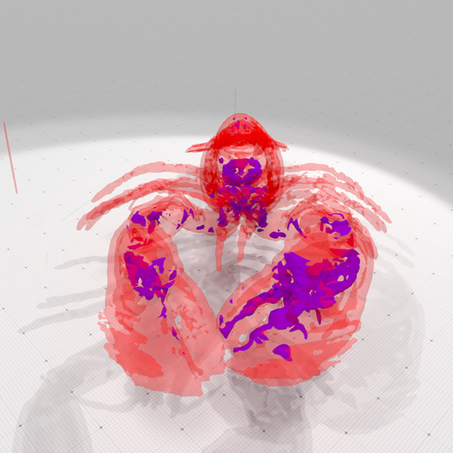
Rendering of lobster 40 (red semi-transparent) and 150 (blue) isosurfaces.

-> build main digital surface -> breadth first traversal -> save OBJ with colored distance.

You may choose your traversal order ("Default", "DepthFirst", "BreadthFirst").

    params( "surfaceTraversal", "BreadthFirst" ) // specifies breadth-first traversal
      ( "colormap", "Jet" ); // specifies the colormap
    auto al_capone = SH3::makeBinaryImage( examplesPath + "samples/Al.100.vol", params );
    auto K         = SH3::getKSpace( al_capone );
    auto surface   = SH3::makeLightDigitalSurface( al_capone, K, params );
    auto surfels   = SH3::getSurfelRange( surface, params );
    auto cmap      = SH3::getColorMap( 0, surfels.size(), params );
    SH3::Colors colors( surfels.size() );
    for ( unsigned int i = 0; i < surfels.size(); ++i ) colors[ i ] = cmap( i );
    bool ok        = SH3::saveOBJ( surface, SH3::RealVectors(), colors, "al-primal-bft.obj" );

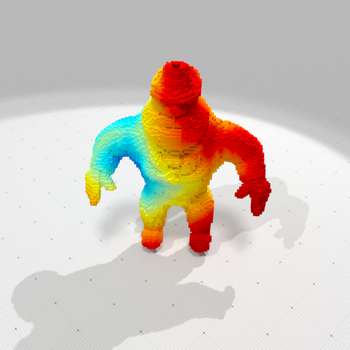
Rendering of Al Capone with a breadth-first traversal colored according to distance (blue to red).

-> build digital surface -> estimate curvatures -> save OBJ.

This example requires ShortcutsGeometry. It shows how tu use the integral invariant curvature estimator on a digital shape model to estimate its mean or Gaussian curvature.

    auto params    = SH3::defaultParameters() | SHG3::defaultParameters();
    params( "colormap", "Tics" );
    auto bimage    = SH3::makeBinaryImage( examplesPath + "samples/Al.100.vol", params );
    auto K         = SH3::getKSpace( bimage, params );
    auto surface   = SH3::makeDigitalSurface( bimage, K, params );
    auto surfels   = SH3::getSurfelRange( surface, params );
    auto curv      = SHG3::getIIMeanCurvatures( bimage, surfels, params );
    // To get Gauss curvatures, write instead:
    // auto curv = SHG3::getIIGaussianCurvatures( bimage, surfels, params );
    auto cmap      = SH3::getColorMap( -0.5, 0.5, params );
    auto colors    = SH3::Colors( surfels.size() );
    std::transform( curv.cbegin(), curv.cend(), colors.begin(), cmap );
    bool ok        = SH3::saveOBJ( surface, SH3::RealVectors(), colors,
                                   "al-H-II.obj" );

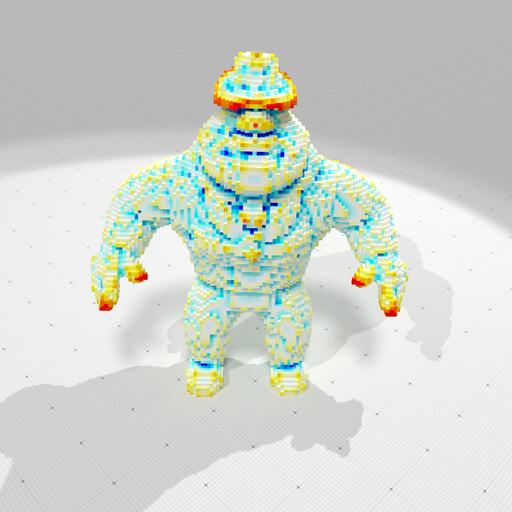
Rendering of Al Capone with estimated mean curvatures (blue is negative, white zero, red is positive, scale is [-0.5, 0.5]).

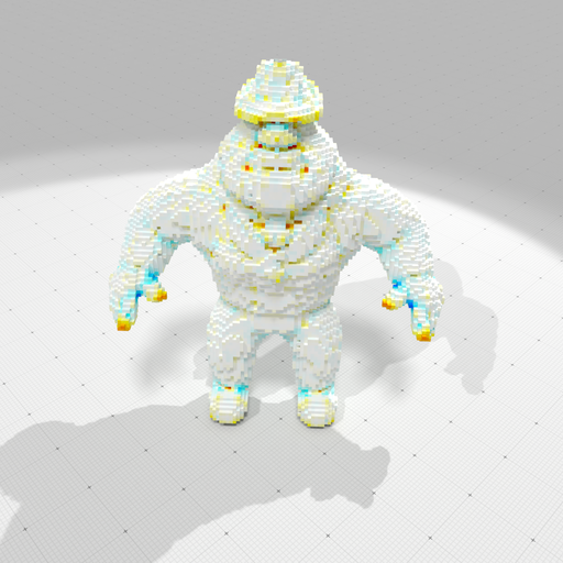
Rendering of Al Capone with estimated Gaus curvatures (blue is negative, white zero, red is positive, scale is [-0.25, 0.25]).

Build polynomial shape -> digitize -> ...

-> noisify -> save as vol file.

    params( "polynomial", "3*x^2+2*y^2+z^2-90" )( "gridstep", 0.25 ) 
      ( "noise", 0.3 );
    auto implicit_shape  = SH3::makeImplicitShape3D( params );
    auto digitized_shape = SH3::makeDigitizedImplicitShape3D( implicit_shape, params );
    auto noisy_shape     = SH3::makeBinaryImage    ( digitized_shape, params );
    auto ok              = SH3::saveBinaryImage    ( noisy_shape, "noisy-ellipsoid.vol" );

-> build surface -> save primal surface as obj

Note: The OBJ file is generally not a combinatorial 2-manifold, since digital surfaces, seen as squares stitched together, are manifold only when they are well-composed.

    params( "polynomial", "goursat" )( "gridstep", 0.25 );
    auto implicit_shape  = SH3::makeImplicitShape3D  ( params );
    auto digitized_shape = SH3::makeDigitizedImplicitShape3D( implicit_shape, params );
    auto K               = SH3::getKSpace( params );
    auto binary_image    = SH3::makeBinaryImage( digitized_shape, params );
    auto surface         = SH3::makeDigitalSurface( binary_image, K, params );
    bool ok              = SH3::saveOBJ( surface, "goursat-primal.obj" );

Rendering of goursat-primal.obj.

-> build indexed surface on a subpart

You may choose which part of a domain is digitized as a binary image, here the first orthant is chosen.

    params( "polynomial", "leopold" )( "gridstep", 0.25 )
      ( "minAABB", -12.0 )( "maxAABB", 12.0 )
      ( "surfaceComponents", "All" );
    auto implicit_shape  = SH3::makeImplicitShape3D  ( params );
    auto digitized_shape = SH3::makeDigitizedImplicitShape3D( implicit_shape, params );
    auto Kwhole          = SH3::getKSpace( params );
    auto K               = SH3::getKSpace( SH3::Point::zero, Kwhole.upperBound(), params );
    auto binary_image    = SH3::makeBinaryImage( digitized_shape, 
                                                 SH3::Domain(K.lowerBound(),K.upperBound()),
                                                 params );
    auto surface         = SH3::makeIdxDigitalSurface( binary_image, K, params );
    trace.info() << "#surfels=" << surface->size() << std::endl;

-> noisify -> count components -> save OBJ with different colors.

    params( "polynomial", "leopold" )( "gridstep", 0.25 )
      ( "minAABB", -12.0 )( "maxAABB", 12.0 )
      ( "surfaceComponents", "All" )( "noise", 0.5 );
    auto implicit_shape  = SH3::makeImplicitShape3D  ( params );
    auto digitized_shape = SH3::makeDigitizedImplicitShape3D( implicit_shape, params );
    auto K               = SH3::getKSpace( params );
    auto binary_image    = SH3::makeBinaryImage(digitized_shape,
                                                SH3::Domain(K.lowerBound(),K.upperBound()),
                                                params );
    // Extracts the whole surface (with all components)
    auto surface         = SH3::makeDigitalSurface( binary_image, K, params );
    // Extracts a vector of connected surfaces.
    auto vec_surfs       = SH3::makeLightDigitalSurfaces( binary_image, K, params );
    trace.info() << "#connected components = " << vec_surfs.size() << std::endl;
    std::map< SH3::Surfel, unsigned int> label;
    unsigned int n = 0;
    for ( auto&& surf : vec_surfs ) {
      auto surfels = SH3::getSurfelRange( surf, params );
      for ( auto&& s : surfels ) label[ s ] = n;
      n += 1;
    }
    auto cmap        = SH3::getColorMap( 0, vec_surfs.size(), params );
    auto all_surfels = SH3::getSurfelRange( surface, params );
    SH3::Colors colors( all_surfels.size() );
    for ( unsigned int i = 0; i < all_surfels.size(); ++i )
      colors[ i ] = cmap( label[ all_surfels[ i ] ] );
    bool ok = SH3::saveOBJ( surface, SH3::RealVectors(), colors, "leopold-primal-cc.obj" );

Rendering of leopold-primal-cc.obj.

-> extract ground-truth geometry

This example requires ShortcutsGeometry. It shows you how to recover ground-truth positions, normal vectors, mean and Gaussian curvatures onto an implicit 3D shape. For each surfel, the geometry is the one of the point nearest to the given surfel centroid.

    params( "polynomial", "3*x^2+2*y^2+z^2-90" )( "gridstep", 0.25 );
    auto implicit_shape  = SH3::makeImplicitShape3D  ( params );
    auto digitized_shape = SH3::makeDigitizedImplicitShape3D( implicit_shape, params );
    auto binary_image    = SH3::makeBinaryImage      ( digitized_shape, params );
    auto K               = SH3::getKSpace( params );
    auto surface         = SH3::makeLightDigitalSurface( binary_image, K, params );
    auto surfels         = SH3::getSurfelRange( surface, params );
    auto positions       = SHG3::getPositions( implicit_shape, K, surfels, params );
    auto normals         = SHG3::getNormalVectors( implicit_shape, K, surfels, params );
    auto mean_curvs      = SHG3::getMeanCurvatures( implicit_shape, K, surfels, params );
    auto gauss_curvs     = SHG3::getGaussianCurvatures( implicit_shape, K, surfels, params );

-> get pointels -> save projected quadrangulated surface.

This example requires ShortcutsGeometry. It shows you how to get pointels from a digital surface and how to project the digital surface onto the given implicit shape.

    const double h       = 0.25;
    params( "polynomial", "goursat" )( "gridstep", h );
    auto implicit_shape  = SH3::makeImplicitShape3D  ( params );
    auto digitized_shape = SH3::makeDigitizedImplicitShape3D( implicit_shape, params );
    auto binary_image    = SH3::makeBinaryImage      ( digitized_shape, params );
    auto K               = SH3::getKSpace( params );
    auto embedder        = SH3::getCellEmbedder( K );
    auto surface         = SH3::makeLightDigitalSurface( binary_image, K, params );
    SH3::Cell2Index c2i;
    auto pointels        = SH3::getPointelRange( c2i, surface );
    SH3::RealPoints pos( pointels.size() );
    std::transform( pointels.cbegin(), pointels.cend(), pos.begin(),
                    [&] (const SH3::Cell& c) { return h * embedder( c ); } ); 
    auto ppos     = SHG3::getPositions( implicit_shape, pos, params );
    bool ok       = SH3::saveOBJ( surface,
                                  [&] (const SH3::Cell& c){ return ppos[ c2i[ c ] ];},
                                  SH3::RealVectors(), SH3::Colors(),
                                  "goursat-quad-proj.obj" );

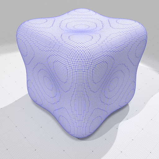
Rendering of goursat-quad-proj.obj with quad edges in blue.

-> extract mean curvature -> save as OBJ with colors

This example requires ShortcutsGeometry. The ground-truth mean curvature is just displayed as a color, using the specified colormap.

    params( "polynomial", "goursat" )( "gridstep", 0.25 )( "colormap", "Tics" );
    auto implicit_shape  = SH3::makeImplicitShape3D  ( params );
    auto digitized_shape = SH3::makeDigitizedImplicitShape3D( implicit_shape, params );
    auto binary_image    = SH3::makeBinaryImage      ( digitized_shape, params );
    auto K               = SH3::getKSpace( params );
    auto surface         = SH3::makeLightDigitalSurface( binary_image, K, params );
    auto surfels         = SH3::getSurfelRange( surface, params );
    auto mean_curv       = SHG3::getMeanCurvatures( implicit_shape, K, surfels, params );
    auto cmap            = SH3::getColorMap( -0.3, 0.3, params );
    auto colors          = SH3::Colors( surfels.size() );
    std::transform( mean_curv.cbegin(), mean_curv.cend(), colors.begin(), cmap );
    bool ok              = SH3::saveOBJ( surface, SH3::RealVectors(), colors,
                                         "goursat-H.obj" );

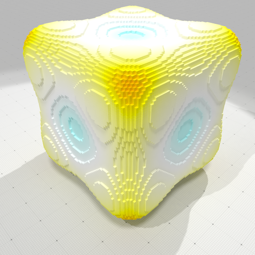
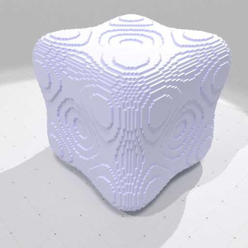
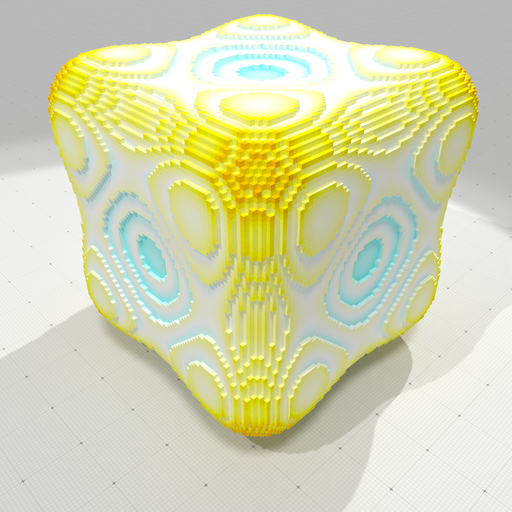
Rendering of goursat-H.obj

-> extract ground-truth and estimated mean curvature -> display errors in OBJ with colors

This example requires ShortcutsGeometry. Both ground-truth and estimated mean curvature are computed. Then you have functions like ShortcutsGeometry::getScalarsAbsoluteDifference and ShortcutsGeometry::getStatistic to measure errors or ShortcutsGeometry::getVectorsAngleDeviation to compare vectors.

    params( "polynomial", "goursat" )( "gridstep", 0.25 )( "colormap", "Tics" )
      ( "R-radius", 5.0 );
    auto implicit_shape  = SH3::makeImplicitShape3D  ( params );
    auto digitized_shape = SH3::makeDigitizedImplicitShape3D( implicit_shape, params );
    auto bimage          = SH3::makeBinaryImage      ( digitized_shape, params );
    auto K               = SH3::getKSpace( params );
    auto surface         = SH3::makeLightDigitalSurface( bimage, K, params );
    auto surfels         = SH3::getSurfelRange( surface, params );
    auto t_curv          = SHG3::getMeanCurvatures( implicit_shape, K, surfels, params );
    auto ii_curv         = SHG3::getIIMeanCurvatures( bimage, surfels, params );
    auto cmap            = SH3::getColorMap( -0.5, 0.5, params );
    auto colors          = SH3::Colors( surfels.size() );
    std::transform( t_curv.cbegin(),  t_curv.cend(),  colors.begin(), cmap );
    bool ok_t  = SH3::saveOBJ( surface, SH3::RealVectors(), colors, "goursat-H.obj" );
    std::transform( ii_curv.cbegin(), ii_curv.cend(), colors.begin(), cmap );
    bool ok_ii = SH3::saveOBJ( surface, SH3::RealVectors(), colors, "goursat-H-ii.obj" );
    auto errors          = SHG3::getScalarsAbsoluteDifference( t_curv, ii_curv );
    auto stat_errors     = SHG3::getStatistic( errors );
    auto cmap_errors     = SH3::getColorMap( 0.0, stat_errors.max(), params );
    std::transform( errors.cbegin(), errors.cend(), colors.begin(), cmap_errors );
    bool ok_err = SH3::saveOBJ( surface, SH3::RealVectors(), colors, "goursat-H-ii-err.obj" );
    trace.info() << "Error Loo=" << SHG3::getScalarsNormLoo( t_curv, ii_curv )
                 << " L1="       << SHG3::getScalarsNormL1 ( t_curv, ii_curv )
                 << " L2="       << SHG3::getScalarsNormL2 ( t_curv, ii_curv )
                 << std::endl;

Ground truth mean curvature

Estimated II mean curvature

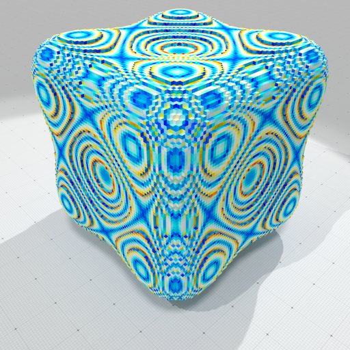
Highlight estimation errors (blue small, red high)

-> build surface -> save primal surface with vcm normals as obj

This example requires ShortcutsGeometry.

Note: The OBJ file is generally not a combinatorial 2-manifold, since digital surfaces, seen as squares stitched together, are manifold only when they are well-composed.

    params( "polynomial", "goursat" )( "gridstep", 0.25 )
      ( "Traversal", "Default" );
    auto implicit_shape  = SH3::makeImplicitShape3D  ( params );
    auto digitized_shape = SH3::makeDigitizedImplicitShape3D( implicit_shape, params );
    auto K               = SH3::getKSpace( params );
    auto binary_image    = SH3::makeBinaryImage( digitized_shape, params );
    auto surface         = SH3::makeDigitalSurface( binary_image, K, params );
    auto surfels         = SH3::getSurfelRange( surface, params );
    auto vcm_normals     = SHG3::getVCMNormalVectors( surface, surfels, params );
    bool ok              = SH3::saveOBJ( surface, vcm_normals, SH3::Colors(),
                                         "goursat-primal-vcm.obj" );

Rendering of goursat-primal.obj (no normals).

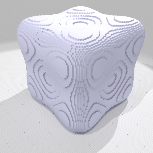
Rendering of goursat-primal-vcm.obj (normals estimated by VCM). Note that staircases effects are still very visible, although normals are good.

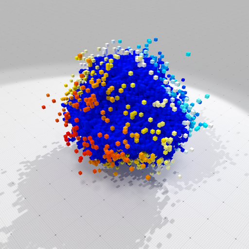
-> digitize implicitly -> estimate II normals and curvature.

This example requires ShortcutsGeometry. You may also analyze the geometry of a digital implicitly defined surface without generating a binary image and only traverse the surface.

    params( "polynomial", "goursat" )( "gridstep", .25 );
    auto implicit_shape  = SH3::makeImplicitShape3D     ( params );
    auto dig_shape       = SH3::makeDigitizedImplicitShape3D( implicit_shape, params );
    auto K               = SH3::getKSpace               ( params );
    auto surface         = SH3::makeDigitalSurface      ( dig_shape, K, params );
    auto surfels         = SH3::getSurfelRange          ( surface, params( "surfaceTraversal", "DepthFirst" ) );
    auto def_surfels     = SH3::getSurfelRange          ( surface, params( "surfaceTraversal", "Default" ) );
    auto ii_normals      = SHG3::getIINormalVectors     ( dig_shape, surfels, params );
    trace.beginBlock( "II with default traversal (slower)" );
    auto ii_mean_curv    = SHG3::getIIMeanCurvatures    ( dig_shape, def_surfels, params );
    trace.endBlock();
    trace.beginBlock( "II with depth-first traversal (faster)" );
    auto ii_mean_curv2   = SHG3::getIIMeanCurvatures    ( dig_shape, surfels, params );
    trace.endBlock();
    auto cmap            = SH3::getColorMap             ( -0.5, 0.5, params );
    auto colors          = SH3::Colors                  ( def_surfels.size() );
    auto match           = SH3::getRangeMatch           ( def_surfels, surfels );
    auto normals         = SH3::getMatchedRange         ( ii_normals, match );
    for ( SH3::Idx i = 0; i < colors.size(); i++ )
      colors[ i ] = cmap( ii_mean_curv[ match[ i ] ] ); 
    bool ok_H  = SH3::saveOBJ( surface, SH3::RealVectors(), colors, "goursat-imp-H-ii.obj" );

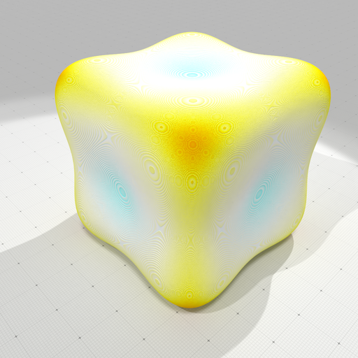
Rendering of goursat-imp-H-ii.obj with a gridstep of 0.03125, more than 2e6 surfels.

Few 2D examples

We give below some minimalistic examples to show that shortcuts can save a lot of lines of code. All examples need at least the following lines:

#include "DGtal/helpers/Stddefs.h"
#include "DGtal/helpers/Shortcuts.h"
...
// Using standard 2D digital space.
typedef Shortcuts<Z2i::KSpace> SH2;
auto params          = SH2::defaultParameters();

Load pgm file -> ...

-> threshold -> save pgm

auto g_image = SH2::makeGrayScaleImage( examplesPath + "samples/contourS.pgm" );
auto b_image = SH2::makeBinaryImage   ( g_image, params( "thresholdMin", 128 ) );
auto ok      = SH2::saveBinaryImage   ( b_image, "contourS-128.pgm" );

Philosophy and naming conventions

Commands are constructed as prefix + type name. Most of them are static methods and are overloaded to accept different set of parameters.

Prefixes

make + Type: means that it will create a new object of type Type and returns it as a smart pointer onto it. Depending on parameters, make can load a file, copy and transform an object, build an empty/not object according to parameters.
make + Type + s: means that it will create new objects of type Type and returns them as a vector of smart pointers onto it.
make + Spec + Type: means that it will create a new object of type Type with some specialized meaning according to Spec and returns it as a smart pointer onto it.
save + Type: means that it will save the pointed object of type Type as a file.
parameters + Type: returns the Parameters object associated to the operations related to the given Type.
get + Type: means that it will return by value an object of type Type.

Types

The following name conventions for types are used. They are defined according to your choice of cellular grid space when defining the Shortcuts type. For instance, if Z3i::KSpace was chosen, then Shortcuts::Point is Z3i::KSpace::Point.

Shortcuts::Point: represents a point with integer coordinates.
Shortcuts::Vector: represents a vector with integer coordinates.
Shortcuts::RealPoint: represents a point with floating-point coordinates.
Shortcuts::RealVector: represents a vector with floating-point coordinates.
Shortcuts::Domain: represents an (hyper-)rectangular digital domain.
Shortcuts::Integer: represents integer numbers (for Point coordinates and Vector components)
Shortcuts::Space: represents a digital space (generally a SpaceND)
Shortcuts::KSpace: represents a cellular grid space (generally a KhalimskySpaceND)
Shortcuts::ImplicitShape3D: represents a functor RealPoint -> Scalar which adds geometry services: isInside, orientation, gradient, meanCurvature, GaussianCurvature, principalCurvatures, nearestPoint
Shortcuts::DigitizedImplicitShape3D: represents the digitization of an ImplicitShape3D as a predicate Point -> bool (isInside), and adds some services: getLowerBound, getUpperBound, embed, round, getDomain, gridSteps, resolution. Note that pixels/voxels are not stored explicitly, so the resolution may be arbirary high.
Shortcuts::BinaryImage: represents a black and white image as an array of bits. It is generally a faster representation of a predicate Point -> bool than an implicit digital shape.
Shortcuts::GrayScaleImage: represents an 8-bits gray-scale image as an array of bytes (unsigned char).
Shortcuts::FloatImage: represents a float image as an array of floats.
Shortcuts::DoubleImage: represents a double image as an array of doubles.
Shortcuts::LightDigitalSurface: represents a connected digital surface over a binary image with an implicit representation.
Shortcuts::DigitalSurface: represents an arbitrary digital surface with an explicit surfel set representation.
Shortcuts::IdxDigitalSurface: represents an indexed digital surface with an explicit array-like representation.
Shortcuts::Mesh: represents a simple mesh with arbitrary faces, but without topology (should be used when no surface topology is needed or when working with non-manifold surfaces).
Shortcuts::TriangulatedSurface: represents a triangulated surface which may have boundaries (use HalfEdgeDataStructure).
Shortcuts::PolygonalSurface: represents a polygonal surface which may have boundaries (use HalfEdgeDataStructure).
Shortcuts::ColorMap: represents a colormap, i.e. a function assigning a color to a real value.

Main methods

General methods
- Shortcuts::defaultParameters: returns the set of all shorcut parameters.
ImplicitShape3D methods
- Shortcuts::getPolynomialList: returns the list of polynomial shapes predefined for implicit shapes
- Shortcuts::parametersImplicitShape3D: parameters related to 3D implicit shapes (polynomial)
- Shortcuts::makeImplicitShape3D: builds a 3D implicit shape
KSpace methods
- Shortcuts::parametersKSpace: parameters related to Khalimsky spaces (closed)
- Shortcuts::getKSpace: overloaded methods for building a Khalimsky space from a domain or an image, from a bounding box, from a digitization process, or from a (indexed or not) digital surface.
- Shortcuts::refKSpace: overloaded methods for referencing the Khalimsky space of a (indexed or not) digital surface.
- Shortcuts::getCellEmbedder: returns the canonic cell embedder of the given space.
- Shortcuts::getSCellEmbedder: returns the canonic signed cell embedder of the given space.
DigitizedImplicitShape3D methods
- Shortcuts::parametersDigitizedImplicitShape3D: parameters related to shape digitization (bounding box, sampling)
- Shortcuts::makeDigitizedImplicitShape3D: digitizes an implicit shape.
BinaryImage methods
- Shortcuts::parametersBinaryImage: parameters related to binary images (noise, threshold).
- Shortcuts::makeBinaryImage: many overloaded methods for creating from scratch, vectorizing shape digitization, loading, copying/noisifying binary images, thresholding gray-scale images.
- Shortcuts::saveBinaryImage: saves a binary image to a file.
GrayScaleImage methods
- Shortcuts::makeGrayScaleImage: overloaded methods for creating from scratch or from binary image, or for loading gray scale images, or for creating a gray-scale image from a float or double image.
- Shortcuts::saveGrayScaleImage: saves a gray scale image to a file.
FloatImage methods
- Shortcuts::makeFloatImage: overloaded methods for creating a float image from a domain or from an implicit shape.
DoubleImage methods
- Shortcuts::makeDoubleImage: overloaded methods for creating a double image from a domain or from an implicit shape.
DigitalSurface methods
- Shortcuts::parametersDigitalSurface: parameters related to digital surfaces (surfel adjacency, components, internal heuristics)
- Shortcuts::getCellEmbedder: returns the canonic cell embedder of the given (indexed or not) digital surface
- Shortcuts::getSCellEmbedder: returns the canonic signed cell embedder of the given (indexed or not) digital surface.
- Shortcuts::makeLightDigitalSurface: creates a light connected surface around a (random) big enough component of a binary image
- Shortcuts::makeLightDigitalSurfaces: creates the vector of all light digital surfaces of the binary image or any one of its big components, can also output representant surfels
- Shortcuts::makeDigitalSurface: creates an arbitrary (connected or not) digital surface from a binary image, from a digitized implicit shape or from an indexed digital surface.
- Shortcuts::makeIdxDigitalSurface: creates an indexed digital surfaces that represents all the boundaries of a binary image or any one of its big components, or any given collection of surfels, or from light digital surface(s).
- Shortcuts::getSurfelRange: returns the surfels of a digital surface in the specified traversal order.
- Shortcuts::getIdxSurfelRange: returns the indexed surfels of an indexed digital surface in the specified traversal order.
- Shortcuts::getPointelRange: returns the pointels of a digital surface in the default order and optionnaly the map Pointel -> Index giving the indices of each pointel, or simply the pointels around a surfel.
- Shortcuts::saveOBJ: saves a digital surface as an OBJ file, with optionally positions, normals and colors information.
Mesh services
- Shortcuts::parametersMesh: parameters related to mesh, triangulated or polygonal surfaces.
- Shortcuts::makeTriangulatedSurface: builds the dual triangulated surface approximating an arbitrary digital surface, or the triangulated surface covering a given mesh, or subdivide a polygonal surface into a triangulated surface, or builds the marching cubes triangulated surface approximating an isosurface in a gray-scale image.
- Shortcuts::makePolygonalSurface: builds a polygonal surface from a mesh, or builds the marching cubes polygonal surface approximating an isosurface in a gray-scale image.
- Shortcuts::makePrimalPolygonalSurface: builds the primal polygonal surface of a digital surface
- Shortcuts::makeDualPolygonalSurface: builds the dual polygonal surface of a digital surface
- Shortcuts::saveOBJ: saves a triangulated or polygonal surface as an OBJ file, with optionnaly normals and colors information.
Utilities
- Shortcuts::parametersUtilities: parameters related to colormaps.
- Shortcuts::getColorMap: returns the specified colormap.
- Shortcuts::getZeroTickedColorMap: returns the specified colormap with a tic around zero.
- Shortcuts::getRangeMatch: returns the perfect or approximate match/correspondence between two ranges.
- Shortcuts::getMatchedRange: returns the perfectly or approximately matched/corresponding range.
- Shortcuts::getPrimalVertices: returns the vertices (possibly consistently ordered along the face) of the given signed cell.
- Shortcuts::outputSurfelsAsObj: outputs surfels in standard OBJ file format.
- Shortcuts::outputPrimalDigitalSurfaceAsObj: outputs any digital surface in standard OBJ file format as its primal quadrangulated mesh.
- Shortcuts::outputPrimalIdxDigitalSurfaceAsObj: outputs any indexed digital surface in standard OBJ file format as its primal quadrangulated mesh.
- Shortcuts::outputDualDigitalSurfaceAsObj: outputs any digital surface in standard OBJ file format as its dual polygonal or triangulated mesh.
ShapeGeometry services
- ShortcutsGeometry::parametersShapeGeometry: parameters related to implicit shape geometry.
- ShortcutsGeometry::getPositions: returns the positions on the 3D implicit shape close to the specified surfels.
- ShortcutsGeometry::getNormalVectors: returns the vectors normal to the 3D implicit shape close to the specified surfels.
- ShortcutsGeometry::getMeanCurvatures: returns the mean curvatures along the 3D implicit shape close to the specified surfels.
- ShortcutsGeometry::getGaussianCurvatures: returns the Gaussian curvatures along the 3D implicit shape close to the specified surfels.
GeometryEstimation services
- ShortcutsGeometry::parametersGeometryEstimation: parameters related to geometric estimators.
- ShortcutsGeometry::getTrivialNormalVectors: returns the trivial (Trivial) normal vectors to the given surfel range
- ShortcutsGeometry::getCTrivialNormalVectors: returns the convolved trivial (CTrivial) normal vectors to the given surfel range
- ShortcutsGeometry::getVCMNormalVectors: returns the Voronoi Covariance Measure (VCM) normal vectors to the given surfel range
- ShortcutsGeometry::getIINormalVectors: returns the Integral Invariant (II) normal vectors to the given surfel range (embedded in a binary image or a digitized implicit shape)
- ShortcutsGeometry::getIIMeanCurvatures: returns the Integral Invariant (II) mean curvatures onto the given surfel range (embedded in a binary image or a digitized implicit shape)
- ShortcutsGeometry::getIIGaussianCurvatures: returns the Integral Invariant (II) Gaussian curvatures onto the given surfel range (embedded in a binary image or a digitized implicit shape)
- ShortcutsGeometry::orientVectors: reorient a range of vectors so as to point in the same half-space as another range of vectors.
- ShortcutsGeometry::getScalarsAbsoluteDifference: return the range of scalars that is the difference of two range of scalars
- ShortcutsGeometry::getVectorsAngleDeviation: return the range of scalars that form the angle deviations between two range of vectors
- ShortcutsGeometry::getStatistic: return the statistic of the given range of values.

Parameters

In all methods, out parameters are listed before in parameters. Also, methods whose result can be influenced by global parameters are parameterized through a Parameters object. Hence static methods follow this pattern:

<return-type> Shortcuts::fonction-name ( [ <out-parameter(s)> ], [ <in-parameter(s)> ], [ Parameters params ] )

The simplest way to get default values for global parameters is to start with a line:

auto params = Shortcuts<KSpace>::defaultParameters();

And then to change your parameter settings with Parameters::operator(), for instance:

params( "gridstep", 0.1 )( "closed", 1 );

You also have the bitwise-or (operator|) to merge Parameters.

Table of Contents

Introduction

Short 3D examples

Load vol file -> ...

-> noisify -> save as vol file.

-> build main connected digital surface

-> extract 2 isosurfaces -> build mesh -> displays them

-> extract 2 triangulated isosurfaces -> save as OBJ

-> build main digital surface -> breadth first traversal -> save OBJ with colored distance.

-> build digital surface -> estimate curvatures -> save OBJ.

Build polynomial shape -> digitize -> ...

-> noisify -> save as vol file.

-> build surface -> save primal surface as obj

-> build indexed surface on a subpart

-> noisify -> count components -> save OBJ with different colors.

-> extract ground-truth geometry

-> get pointels -> save projected quadrangulated surface.

-> extract mean curvature -> save as OBJ with colors

-> extract ground-truth and estimated mean curvature -> display errors in OBJ with colors

-> build surface -> save primal surface with vcm normals as obj

-> digitize implicitly -> estimate II normals and curvature.

Few 2D examples

Load pgm file -> ...

-> threshold -> save pgm

Philosophy and naming conventions

Prefixes

Types

Main methods

Parameters